I recently got to use a very curious Haskell technique [note: As production as research code gets, anyway! ] time traveling. I say this with the utmost seriousness. This technique worked like magic for the problem I was trying to solve, and so I thought I’d share what I learned. In addition to the technique and its workings, I will also explain how time traveling can be misused, yielding computations that never terminate.
Time Traveling
Some time ago, I read this post by Csongor Kiss about time traveling in Haskell. It’s really cool, and makes a lot of sense if you have wrapped your head around lazy evaluation. I’m going to present my take on it here, but please check out Csongor’s original post if you are interested.
Say that you have a list of integers, like [3,2,6]. Next, suppose that
you want to find the maximum value in the list. You can implement such
behavior quite simply with pattern matching:
myMax :: [Int] -> Int
myMax [] = error "Being total sucks"
myMax (x:xs) = max x $ myMax xs
You could even get fancy with a fold:
myMax :: [Int] -> Int
myMax = foldr1 max
All is well, and this is rather elementary Haskell. But now let’s look at
something that Csongor calls the repMax problem:
Imagine you had a list, and you wanted to replace all the elements of the list with the largest element, by only passing the list once.
How can we possibly do this in one pass? First, we need to find the maximum element, and only then can we have something to replace the other numbers with! It turns out, though, that we can just expect to have the future value, and all will be well. Csongor provides the following example:
repMax :: [Int] -> Int -> (Int, [Int])
repMax [] rep = (rep, [])
repMax [x] rep = (x, [rep])
repMax (l : ls) rep = (m', rep : ls')
  where (m, ls') = repMax ls rep
        m' = max m l
In this example, repMax takes the list of integers,
each of which it must replace with their maximum element.
It also takes as an argument the maximum element,
as if it had already been computed. It does, however,
still compute the intermediate maximum element,
in the form of m'. Otherwise, where would the future
value even come from?
Thus far, nothing too magical has happened. It’s a little
strange to expect the result of the computation to be
given to us; it just looks like wishful
thinking. The real magic happens in Csongor’s doRepMax
function:
doRepMax :: [Int] -> [Int]
doRepMax xs = xs'
  where (largest, xs') = repMax xs largest
Look, in particular, on the line with the where clause.
We see that repMax returns the maximum element of the
list, largest, and the resulting list xs' consisting
only of largest repeated as many times as xs had elements.
But what’s curious is the call to repMax itself. It takes
as input xs, the list we’re supposed to process… and
largest, the value that it itself returns.
This works because Haskell’s evaluation model is, effectively, lazy graph reduction. That is, you can think of Haskell as manipulating your code as [note: Why is it called graph reduction, you may be wondering, if the runtime is manipulating syntax trees? To save on work, if a program refers to the same value twice, Haskell has both of those references point to the exact same graph. This violates the tree's property of having only one path from the root to any node, and makes our program a DAG (at least). Graph nodes that refer to themselves (which are also possible in the model) also violate the properties of a a DAG, and thus, in general, we are working with graphs. ] performing substitutions and simplifications as necessary until it reaches a final answer. What the lazy part means is that parts of the syntax tree that are not yet needed to compute the final answer can exist, unsimplified, in the tree. Why don’t we draw a few graphs to get familiar with the idea?
Visualizing Graphs and Their Reduction
A word of caution: the steps presented below may significantly differ from the actual graph reduction algorithms used by modern compilers. In particular, this section draws a lot of ideas from Simon Peyton Jones’ book, Implementing functional languages: a tutorial. However, modern functional compilers (i.e. GHC) use a much more complicated abstract machine for evaluating graph-based code, based on – from what I know – the spineless tagless G-machine. In short, this section, in order to build intuition, walks through how a functional program evaluated using graph reduction may behave; the actual details depend on the compiler.
Let’s start with something that doesn’t have anything fancy. We can take a look at the graph of the expression:
length [1]
Stripping away Haskell’s syntax sugar for lists, we can write this expression as:
length (1:[])
Then, recalling that (:), or ‘cons’, is just a binary function, we rewrite:
length ((:) 1 [])
We’re now ready to draw the graph; in this case, it’s pretty much identical to the syntax tree of the last form of our expression:
![The initial graph of length [1].](/blog/haskell_lazy_evaluation/length_1.png)
The initial graph of length [1].
In this image, the @ nodes represent function application. The
root node is an application of the function length to the graph that
represents the list [1]. The list itself is represented using two
application nodes: (:) takes two arguments, the head and tail of the
list, and function applications in Haskell are
curried. Eventually,
in the process of evaluation, the body of length will be reached,
and leave us with the following graph:
![The graph of length [1] after the body of length is expanded.](/blog/haskell_lazy_evaluation/length_2.png)
The graph of length [1] after the body of length is expanded.
Conceptually, we only took one reduction step, and thus, we haven’t yet gotten
to evaluating the recursive call to length. Since (+)
is also a binary function, 1+length xs is represented in this
new graph as two applications of (+), first to 1, and then
to length [].
But what is that box at the root? This box used to be the root of the first graph, which was an application node. However, it is now a an indirection. Conceptually, reducing this indirection amounts to reducing the graph it points to. But why have we [note: This is a key aspect of implementing functional languages. The language itself may be pure, while the runtime can be, and usually is, impure and stateful. After all, computers are impure and stateful, too! ] in this manner? Because Haskell is a pure language, of course! If we know that a particular graph reduces to some value, there’s no reason to reduce it again. However, as we will soon see, it may be used again, so we want to preserve its value. Thus, when we’re done reducing a graph, we replace its root node with an indirection that points to its result.
When can a graph be used more than once? Well, how about this:
let x = square 5 in x + x
Here, the initial graph looks as follows:
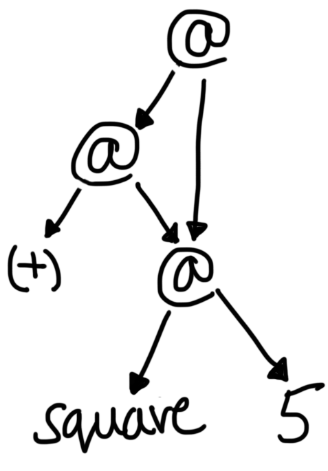
The initial graph of let x = square 5 in x + x.
As you can see, this is a graph, but not a tree! Since both
variables x refer to the same expression, square 5, they
are represented by the same subgraph. Then, when we evaluate square 5
for the first time, and replace its root node with an indirection,
we end up with the following:
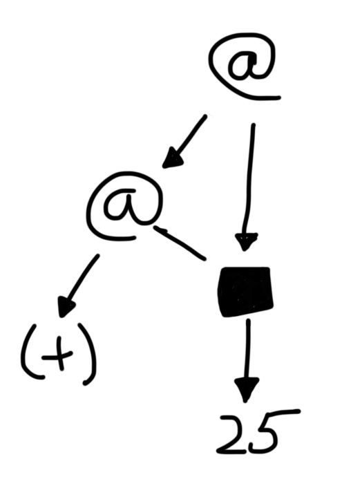
The graph of let x = square 5 in x + x after square 5 is reduced.
There are two 25s in the graph, and no more squares! We only
had to evaluate square 5 exactly once, even though (+)
will use it twice (once for the left argument, and once for the right).
Our graphs can also include cycles.
A simple, perhaps the most simple example of this in practice is Haskell’s
fix function. It computes a function’s fixed point,
[note:
In fact, in the lambda calculus, fix is pretty much the only
way to write recursive functions. In the untyped lambda calculus, it can
be written as:
In the simply typed lambda calculus, it cannot be written in any way, and
needs to be added as an extension, typically written as .
]
It’s implemented as follows:
fix f = let x = f x in x
See how the definition of x refers to itself? This is what
it looks like in graph form:
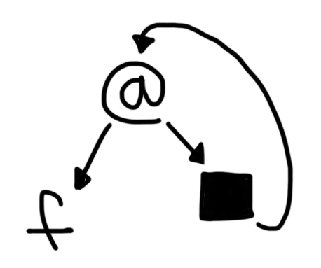
The initial graph of let x = f x in x.
I think it’s useful to take a look at how this graph is processed. Let’s
pick f = (1:). That is, f is a function that takes a list,
and prepends 1 to it. Then, after constructing the graph of f x,
we end up with the following:
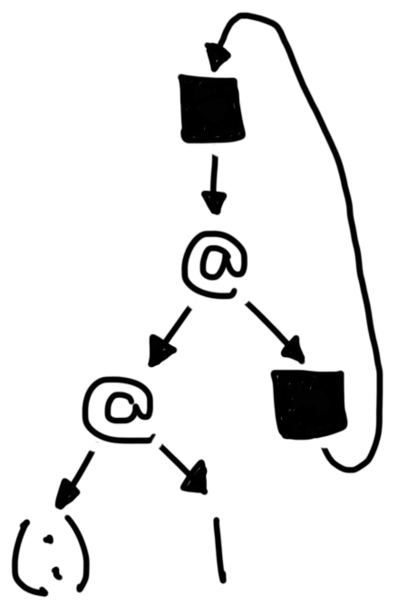
The graph of fix (1:) after it’s been reduced.
We see the body of f, which is the application of (:) first to the
constant 1, and then to f’s argument (x, in this case). As
before, once we evaluated f x, we replaced the application with
an indirection; in the image, this indirection is the top box. But the
argument, x, is itself an indirection which points to the root of f x,
thereby creating a cycle in our graph. Traversing this graph looks like
traversing an infinite list of 1s.
Almost there! A node can refer to itself, and, when evaluated, it
is replaced with its own value. Thus, a node can effectively reference
its own value! The last piece of the puzzle is how a node can access
parts of its own value: recall that doRepMax calls repMax
with only largest, while repMax returns (largest, xs').
I have to admit, I don’t know the internals of GHC, but I suspect
this is done by translating the code into something like:
doRepMax :: [Int] -> [Int]
doRepMax xs = snd t
  where t = repMax xs (fst t)
Detailed Example: Reducing doRepMax
If the above examples haven’t elucidated how doRepMax works,
stick around in this section and we will go through it step-by-step.
This is a rather long and detailed example, so feel free to skip
this section to read more about actually using time traveling.
If you’re sticking around, why don’t we watch how the graph of doRepMax [1, 2] unfolds.
This example will be more complex than the ones we’ve seen
so far; to avoid overwhelming ourselves with notation,
let’s adopt a different convention of writing functions. Instead
of using application nodes @, let’s draw an application of a
function f to arguments x1 through xn as a subgraph with root f
and children xs. The below figure demonstrates what I mean:
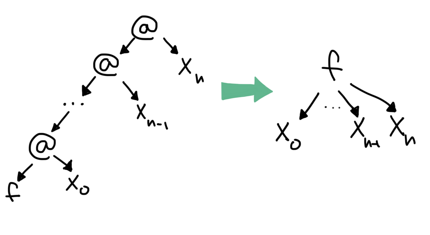
The new visual notation used in this section.
Now, let’s write the initial graph for doRepMax [1,2]:
![The initial graph of doRepMax [1,2].](/blog/haskell_lazy_evaluation/repmax_1.png)
The initial graph of doRepMax [1,2].
Other than our new notation, there’s nothing too surprising here.
The first step of our hypothetical reduction would replace the application of doRepMax with its
body, and create our graph’s first cycle. At a high level, all we want is the second element of the tuple
returned by repMax, which contains the output list. To get
the tuple, we apply repMax to the list [1,2] and the first element
of its result. The list [1,2] itself
consists of two uses of the (:) function.
![The first step of reducing doRepMax [1,2].](/blog/haskell_lazy_evaluation/repmax_2.png)
The first step of reducing doRepMax [1,2].
Next, we would also expand the body of repMax. In
the following diagram, to avoid drawing a noisy amount of
crossing lines, I marked the application of fst with
a star, and replaced the two edges to fst with
edges to similar looking stars. This is merely
a visual trick; an edge leading to a little star is
actually an edge leading to fst. Take a look:
![The second step of reducing doRepMax [1,2].](/blog/haskell_lazy_evaluation/repmax_3.png)
The second step of reducing doRepMax [1,2].
Since (,) is a constructor, let’s say that it doesn’t
need to be evaluated, and that its
[note:
A graph that can't be reduced further is said to be in normal form,
by the way.
]
(in practice, other things like
packing may occur here, but they are irrelevant to us).
If (,) can’t be reduced, we can move on to evaluating snd. Given a pair, snd
simply returns the second element, which in our
case is the subgraph starting at (:). We
thus replace the application of snd with an
indirection to this subgraph. This leaves us
with the following:
![The third step of reducing doRepMax [1,2].](/blog/haskell_lazy_evaluation/repmax_4.png)
The third step of reducing doRepMax [1,2].
Since it’s becoming hard to keep track of what part of the graph
is actually being evaluated, I marked the former root of doRepMax [1,2] with
a blue star. If our original expression occured at the top level,
the graph reduction would probably stop here. After all,
we’re evaluating our graphs using call-by-need, and there
doesn’t seem to be a need for knowing the what the arguments of (:) are.
However, stopping at (:) wouldn’t be very interesting,
and we wouldn’t learn much from doing so. So instead, let’s assume
that something is trying to read the elements of our list;
perhaps we are trying to print this list to the screen in GHCi.
In this case, our mysterious external force starts unpacking and
inspecting the arguments to (:). The first argument to (:) is
the list’s head, which is the subgraph starting with the starred application
of fst. We evaluate it in a similar manner to snd. That is,
we replace this fst with an indirection to the first element
of the argument tuple, which happens to be the subgraph starting with max:
![The fourth step of reducing doRepMax [1,2].](/blog/haskell_lazy_evaluation/repmax_5.png)
The fourth step of reducing doRepMax [1,2].
Phew! Next, we need to evaluate the body of max. Let’s make one more
simplification here: rather than substitututing max for its body
here, let’s just reason about what evaluating max would entail.
We would need to evaluate its two arguments, compare them,
and return the larger one. The argument 1 can’t be reduced
any more (it’s just a number!), but the second argument,
a call to fst, needs to be processed. To do so, we need to
evaluate the call to repMax. We thus replace repMax
with its body:
![The fifth step of reducing doRepMax [1,2].](/blog/haskell_lazy_evaluation/repmax_6.png)
The fifth step of reducing doRepMax [1,2].
We’ve reached one of the base cases here, and there
are no more calls to max or repMax. The whole reason
we’re here is to evaluate the call to fst that’s one
of the arguments to max. Given this graph, doing so is easy.
We can clearly see that 2 is the first element of the tuple
returned by repMax [2]. We thus replace fst with
an indirection to this node:
![The sixth step of reducing doRepMax [1,2].](/blog/haskell_lazy_evaluation/repmax_7.png)
The sixth step of reducing doRepMax [1,2].
This concludes our task of evaluating the arguments to max.
Comparing them, we see that 2 is greater than 1, and thus,
we replace max with an indirection to 2:
![The seventh step of reducing doRepMax [1,2].](/blog/haskell_lazy_evaluation/repmax_8.png)
The seventh step of reducing doRepMax [1,2].
The node that we starred in our graph is now an indirection (the
one that used to be the call to fst) which points to
another indirection (formerly the call to max), which
points to 2. Thus, any edge pointing to a star now
points to the value 2.
By finding the value of the starred node, we have found the first
argument of (:), and returned it to our mysterious external force.
If we were printing to GHCi, the number 2 would appear on the screen
right about now. The force then moves on to the second argument of (:),
which is the call to snd. This snd is applied to an instance of (,), which
can’t be reduced any further. Thus, all we have to do is take the second
element of the tuple, and replace snd with an indirection to it:
![The eighth step of reducing doRepMax [1,2].](/blog/haskell_lazy_evaluation/repmax_9.png)
The eighth step of reducing doRepMax [1,2].
The second element of the tuple was a call to (:), and that’s what the mysterious
force is processing now. Just like it did before, it starts by looking at the
first argument of this list, which is the list’s head. This argument is a reference to
the starred node, which, as we’ve established, eventually points to 2.
Another 2 pops up on the console.
Finally, the mysterious force reaches the second argument of the (:),
which is the empty list. The empty list also cannot be evaluated any
further, so that’s what the mysterious force receives. Just like that,
there’s nothing left to print to the console. The mysterious force ceases.
After removing the unused nodes, we are left with the following graph:
![The result of reducing doRepMax [1,2].](/blog/haskell_lazy_evaluation/repmax_10.png)
The result of reducing doRepMax [1,2].
As we would have expected, two 2s were printed to the console, and our
final graph represents the list [2,2].
Using Time Traveling
Is time tarveling even useful? I would argue yes, especially in cases where Haskell’s purity can make certain things difficult.
As a first example, Csongor provides an assembler that works in a single pass. The challenge in this case is to resolve jumps to code segments occuring after the jump itself; in essence, the address of the target code segment needs to be known before the segment itself is processed. Csongor’s code uses the Tardis monad, which combines regular state, to which you can write and then later read from, and future state, from which you can read values before your write them. Check out his complete example here.
Alternatively, here’s an example from my research, which my
coworker and coauthor Kai helped me formulate. I’ll be fairly
vague, since all of this is still in progress. The gist is that
we have some kind of data structure (say, a list or a tree),
and we want to associate with each element in this data
structure a ‘score’ of how useful it is. There are many possible
heuristics of picking ‘scores’; a very simple one is
to make it inversely propertional to the number of times
an element occurs. To be more concrete, suppose
we have some element type Element:
|
|
Suppose also that our data structure is a binary tree:
|
|
We then want to transform an input ElementTree, such as:
Node A (Node A Empty Empty) Empty
Into a scored tree, like:
Node (A,0.5) (Node (A,0.5) Empty Empty) Empty
Since A occured twice, its score is 1/2 = 0.5.
Let’s define some utility functions before we get to the meat of the implementation:
|
|
The addElement function simply increments the counter for a particular
element in the map, adding the number 1 if it doesn’t exist. The getScore
function computes the score of a particular element, defaulting to 1.0 if
it’s not found in the map.
Just as before – noticing that passing around the future values is getting awfully bothersome – we write our scoring function as though we have a ‘future value’.
|
|
The actual doAssignScores function is pretty much identical to
doRepMax:
|
|
There’s quite a bit of repetition here, especially in the handling
of future values - all of our functions now accept an extra
future argument, and return a work-in-progress future value.
This is what the Tardis monad, and its corresponding
TardisT monad transformer, aim to address. Just like the
State monad helps us avoid writing plumbing code for
forward-traveling values, Tardis helps us do the same
for backward-traveling ones.
Cycles in Monadic Bind
We’ve seen that we’re able to write code like the following:
(a, b) = f a c
That is, we were able to write function calls that referenced
their own return values. What if we try doing this inside
a do block? Say, for example, we want to sprinkle some time
traveling into our program, but don’t want to add a whole new
transformer into our monad stack. We could write code as follows:
do
    (a, b) <- f a c
    return b
Unfortunately, this doesn’t work. However, it’s entirely
possible to enable this using the RecursiveDo language
extension:
{-# LANGUAGE RecursiveDo #-}
Then, we can write the above as follows:
do
    rec (a, b) <- f a c
    return b
This power, however, comes at a price. It’s not as straightforward
to build graphs from recursive monadic computations; in fact,
it’s not possible in general. The translation of the above
code uses MonadFix. A monad that satisfies MonadFix has
an operation mfix, which is the monadic version of the fix
function we saw earlier:
mfix :: Monad m => (a -> m a) -> m a
-- Regular fix, for comparison
fix :: (a -> a) -> a
To really understand how the translation works, check out the paper on recursive do notation.
Beware The Strictness
Though Csongor points out other problems with the
time traveling approach, I think he doesn’t mention
an important idea: you have to be very careful about introducing
strictness into your programs when running time-traveling code.
For example, suppose we wanted to write a function,
takeUntilMax, which would return the input list,
cut off after the first occurence of the maximum number.
Following the same strategy, we come up with:
|
|
In short, if we encounter our maximum number, we just return a list of that maximum number, since we do not want to recurse further. On the other hand, if we encounter a number that’s not the maximum, we continue our recursion.
Unfortunately, this doesn’t work; our program never terminates. You may be thinking:
Well, obviously this doesn’t work! We didn’t actually compute the maximum number properly, since we stopped recursing too early. We need to traverse the whole list, and not just the part before the maximum number.
To address this, we can reformulate our takeUntilMax
function as follows:
|
|
Now we definitely compute the maximum correctly! Alas,
this doesn’t work either. The issue lies on lines 5 and 18,
more specifically in the comparison x == m. Here, we
are trying to base the decision of what branch to take
on a future value. This is simply impossible; to compute
the value, we need to know the value!
This is no ‘silly mistake’, either! In complicated programs
that use time traveling, strictness lurks behind every corner.
In my research work, I was at one point inserting a data structure into
a set; however, deep in the structure was a data type containing
a ‘future’ value, and using the default Eq instance!
Adding the data structure to a set ended up invoking (==) (or perhaps
some function from the Ord typeclass),
which, in turn, tried to compare the lazily evaluated values.
My code therefore didn’t terminate, much like takeUntilMax.
Debugging time traveling code is, in general,
a pain. This is especially true since future values don’t look any different
from regular values. You can see it in the type signatures
of repMax and takeUntilMax: the maximum number is just an Int!
And yet, trying to see what its value is will kill the entire program.
As always, remember Brian W. Kernighan’s wise words:
Debugging is twice as hard as writing the code in the first place. Therefore, if you write the code as cleverly as possible, you are, by definition, not smart enough to debug it.
Conclusion
This is about it! In a way, time traveling can make code performing certain operations more expressive. Furthermore, even if it’s not groundbreaking, thinking about time traveling is a good exercise to get familiar with lazy evaluation in general. I hope you found this useful!